Modeling Basal Flow in Comsol
Introduction
Our goal was to develop a COMSOL model for the bottom channel of the µSiM that can be accessed and easily used by anyone with a COMSOL license. Previously developed simulations for the µSiM rely on the CAD import module, which can introduce unnecessary complications with regards to accessibility and ease-of-use, particularly to expand upon or adapt models. To facilitate the sharing of COMSOL with all collaborators, we re-created the bottom channel geometry of the µSiM using COMSOL’s built in geometry capabilities, then followed the typical workflow of defining our materials, boundaries, and physics before running the study.
COMSOL Model Access
We first tried to adapt a previously developed COMSOL model for the bottom channel. Though the simulation ran as expected when we use the CAD Import Module, which is a paid add-on for COMSOL, we confirmed that there was no way to use the model or its geometry with a regular COMSOL license. This is problematic because 3D meshes for the channel geometry must be manually corrected before they can be used for simulations and this process may introduce loss. Moreover, it is far more challenging to assign precise boundary conditions to imported 3D models due to the way that COMSOL converts meshes to geometrical entities. Our attempts to import simple STL, STEP, DXF files, and other formats all led to errors in COMSOL.
To avoid dependence on COMSOL paid add-on modules, we re-created the geometry of the µSiM bottom channel in COMSOL directly and saved it as MPH or MPHBIN format which store the entire model or more specific selections such as geometry, respectively. This ensures that the simulation can be directly shared with all collaborators of TraCe-bMPS.
Physics
For the first iteration of the model, I treated the membrane and all channel walls as impermeable boundaries. The flow injection port was treated as a fluidic inlet, and the opposite port was treated as a fluidic outlet. We simulated laminar flow to assess shear stress, velocity, and pressure near a trench-down membrane exposed to bottom channel flow at varying inlet flow rates. We expect that this simulation is representative of the shear forces that affect cells seeded on the underside of a nanomembrane.
Due to the no-slip boundary condition we must consider velocity at the surface of the membrane to be 0. This is the default assumption at a boundary for laminar and turbulent flow simulations in COMSOL – no selections are needed.
The flow rate (LFR) is set in the inlet to 96 uL/min (based on our real-world calibrations – LFR is the lowest flow rate we achieved on our setup). We plotted velocity and shear results for whole-channel measurements (volumetric or sliced) or membrane trench measurements (volumetric or sliced).
Boundary Conditions
I’ve created two models, one for a trench up and trench-down configuration. Should you wish to make any modifications, it may be easiest to first look at the global parameters tab where sizes used for the design are defined, then “rebuild” your geometry to reflect these changes in the model before re-running any studies. The boundaries are defined for each physics, so you can find these on the left-hand side under “laminar flow” physics. The other two physics are disabled so you don’t need to consider those boundaries unless expanding the model.
Results
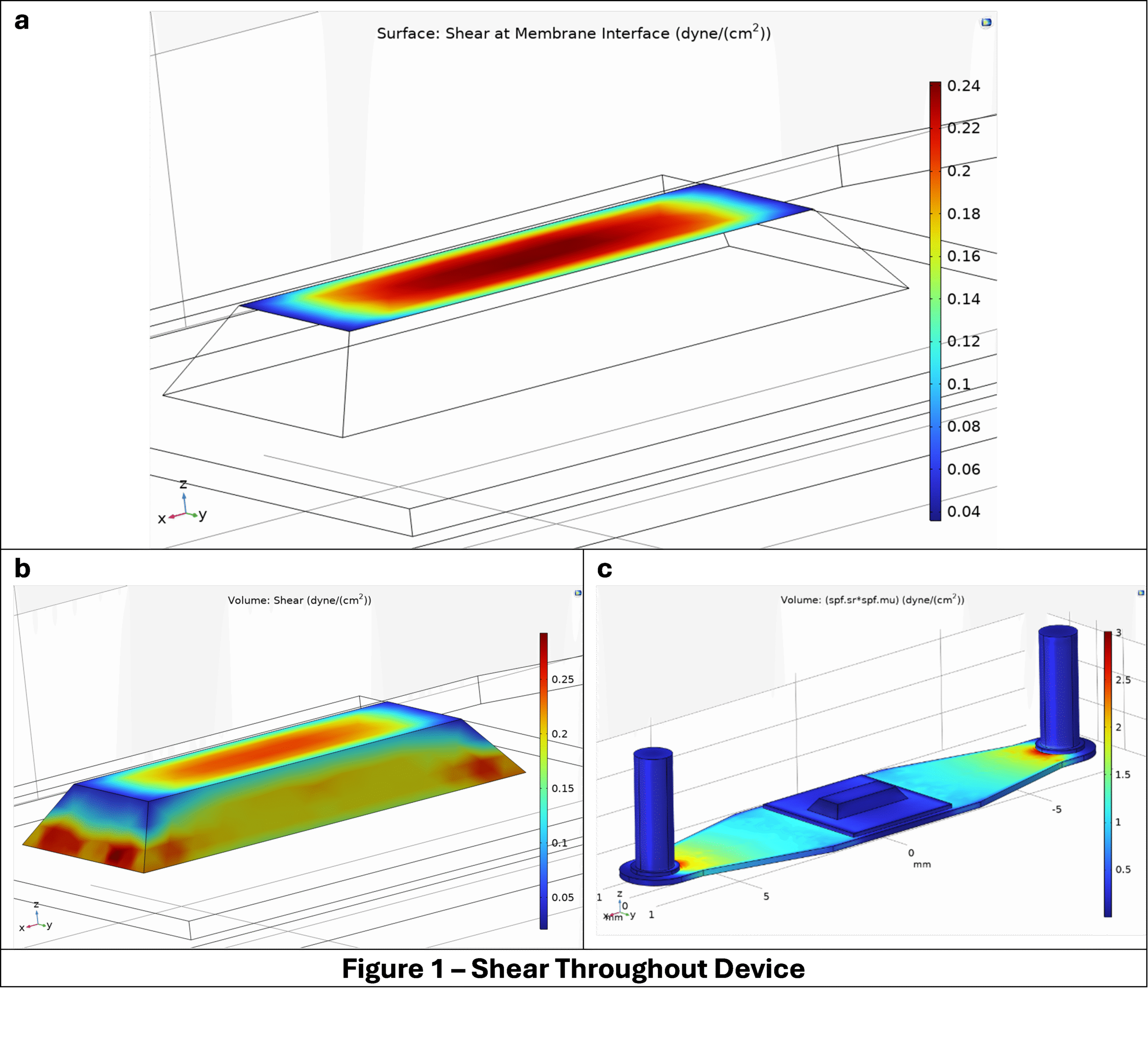
Screenshots from our initial studies are below. Note that we have a pre-set camera view but if you change the camera position you can re-center it by “building” with the camera selected on the left-hand side.

We can see here that the shear around the membrane is minimal in comparison to the stresses that will be experienced around our inlets and outlets – indicating the importance of the consideration of local forces in complex devices over bulk transport to allow for improved physiological relevance.
Shear on ARPE-19 cells is not well studied, but an in-vitro study used less than 10 dynes of various ranges (1).
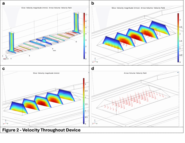
Here we have created slices throughout the device spaced such that the profile along the center of the inlet is revealed and each level has a few profiles. The device gets thicker moving into the middle layer, and thicker once more when expanding into the trench so it follows that the velocity within the trench region is comparatively lower. Comparing this to our shear from earlier, we can see that it makes sense that the edges of the trench have less shear based on our vectors flowing along the path of least resistance.
Summary
This model allows for us to monitor shear stress and other transport properties throughout the device and specifically against the membrane within the trench area. This can be expanded to serve many functions, but initially allows for us to determine what shear stress our cells are exposed to as a function of flow rate to enable better understanding and control of experimental parameters.
Future Work
Implementation of transfer of dilute species (tds) and brinkman equations is readily available in this model by re-defining the boundaries. For tds we can look at fluorescent movement, bead tracking, antibody transfer, etc. throughout the entire device. Previously we looked at permeability from a static top of membrane down through approach, but we also are interested in as we flow something through the bottom how much permeates up through into the top channel in various conditions.
We can apply brinkman equations for the membranes assuming they have no thickness. We can test permeability between – 1 x 10 ^-2 to 1 x 10^-5 cm/min based on previous testing by Kevin Ling.
Additionally, we want to do a parametric sweep as a function of flow rate – we are still comparing our flow rate (96uL/min) to the flow rate of others in the group and can see what flow rate gives a desirable shear. We can also try various flow rates to determine what rate gives the shear we desire.
Calibration
I – Peristaltic Pumps
Peristaltic Pumps are quantified based on rotations per minute, but it is important to note that resistance of the up or downstream fluids and most notably, the diameter of tubing inside the pump will have a great influence on flow rate by affecting the fluid displaced per revolution. Thus, for each pump and each new setup it is important to quantify the flow rate used in a standardized manner. For this setup, I’ve quantified 1 RPM to be approximately 96 uL/min with Masterflex 1/16″ ID x 1/8″ OD Tubing. As we can’t do this in a loop, I introduced an additional large falcoln tube to feed into the smaller transfer tube to have some degree of backpressure or “pulling” as it would in the loop – but this is an approximation. It then was fed into a larger tube and calibrated 20 mL at a time.
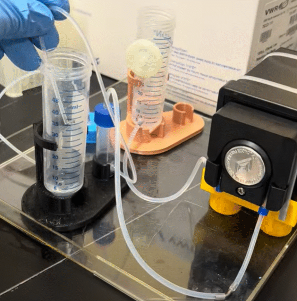 |
| Figure 3 – Flow Rate Calibration |
II – Membrane Permeability
This was tested using the protocol described by Molly McCloskey (2) where we have a fluorescent dye in the top well, allow it to sit for some time, then use a 50uL microwell in the bottom-channel inlet then pull 50uL out of the outlet to then be quantified. We did not utilize this, but I’ve included it for future work where we consider transfer across the membrane in our model.
References
- Duan, Sujuan, Yingjie Li, Yanyan Zhang, Xuan Zhu, Yan Mei, Dongmei Xu, and Guofu Huang. “The Response of Corneal Endothelial Cells to Shear Stress in an In Vitro Flow Model.” Journal of Ophthalmology 2021 (November 27, 2021): 9217866. https://doi.org/10.1155/2021/9217866.
- McCloskey, Molly C., Pelin Kasap, S. Danial Ahmad, Shiuan‐Haur Su, Kaihua Chen, Mehran Mansouri, Natalie Ramesh, et al. “The Modular µSiM: A Mass Produced, Rapidly Assembled, and Reconfigurable Platform for the Study of Barrier Tissue Models In Vitro.” Advanced Healthcare Materials 11, no. 18 (September 2022): 2200804. https://doi.org/10.1002/adhm.202200804.
- See the other blog post for related information applied toward testing flow bumpers.