In this article we’ll share some of our preliminary results regarding the parameters of the NPN device. We will also be making some recommendations for further tuning of the design to specific tasks.

We will be comparing one of the more recent batches to the one used in the Nano Letters paper. Note that for the calculations carried out in the sections below we’ve assumed a circular cross sectional area for the pores and ignored any sagging of the filter layer that may have been present

Parameter Changes

A number of changes were made to the parameters in order to facilitate certain tasks. Those relevant to this discussion are recounted in the table below.

Parameter	Batch A	Batch B
Average filter pore radius	25 nm	12 nm
Average sensing pore radius	7.5 nm	5 nm
Spacer radius	500 nm	1500 nm
Spacer length	200 nm	800 nm
Average porosity	5%	16%

From electrostatics we know that the flux must be conserved across the device as prescribed by,

We can immediately see that one effect of the changes in these parameters is going to be a great reduction to the magnitude of the electric field in the NPN layer (roughly 100 times weaker).
In addition to the parameters of the NPN being changed the range of molecule lengths studied changed. The longest molecule has a contour length of 7000 bp (~ 2380 nm). Assuming the Kratky-Porod model and persistence length of dsDNA in 4M Li solvent (~30nm) the radius of gyration of this molecule is ~ 150nm. We’ll be using this molecule for our calculations as it is of experimental interest.

A toy model for bending

Our first approach is some modelling on the likelihood of translocation. Due to the reduced field in each individual filter pore as well as the smaller pore size we want to know if it is possible to even begin the translocation process. We begin by making the assumption that if a molecule can fold through a pore in a reasonable time then it can most certainly begin single file translocation in a reasonable time. As such, we will study the case where a chain folds through a pore. In the energy barrier limited picture this implies that in order to have successful translocation the electric energy exerted on a segment of the chain needs to be greater than(or within fluctuation of) bending energy of the chain. From these considerations we can construct a rough (and fairly minimal) model for bending through a pore in the  limit. We consider a hyperbola parameterized by . We use the length of the semi-minor axis  for the pore radius  as keeping it fixed while changing the length of the semi-major axis  will “bend” the hyperbola. One limitation of the model that is immediately obvious is that the free ends always point outwards instead of also bending. We term this an appropriate approximation as we only need a model to satisfy the fact that a segment of the chain is folded while the ends go away from the pore. As a result this calculation provides a lower bound to the bending energy. A pictorial representation of the system is shown in the schematic below.

 

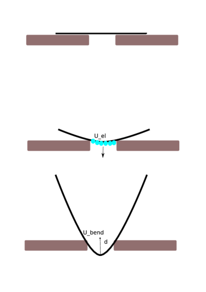
The bending energy of a polymer chain modelled as a continuous curve is given by,

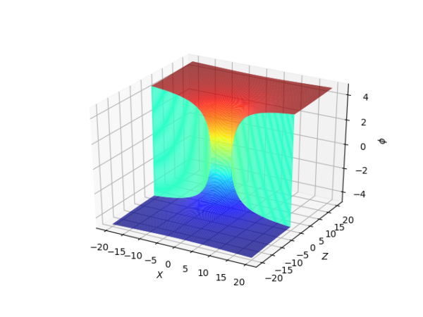
where  is the persistence length of the chain,  is the contour length and  is the unit vector obtained from the tangent vector, . For the electric field driving the chain we use a potential in oblate spheroid coordinates defined as,

where  is the radius of the pore. This potential models the field through a pore as shown in the figure below (it also captures the field far from the pore).

Analysis

Equipped with the equations of the preceding section we can compute the bending and electric energies for the parameter sets in table above. We will also be comparing the bending energies with those obtained from simulations for partial validation. For the sake of making the comparison easier we will be using simulation units. The energy units in our simulations are defined by . The length scale is defined by . We define a correspondence between the length scales of the simulation and those of the experiment by setting  = 5 nm.

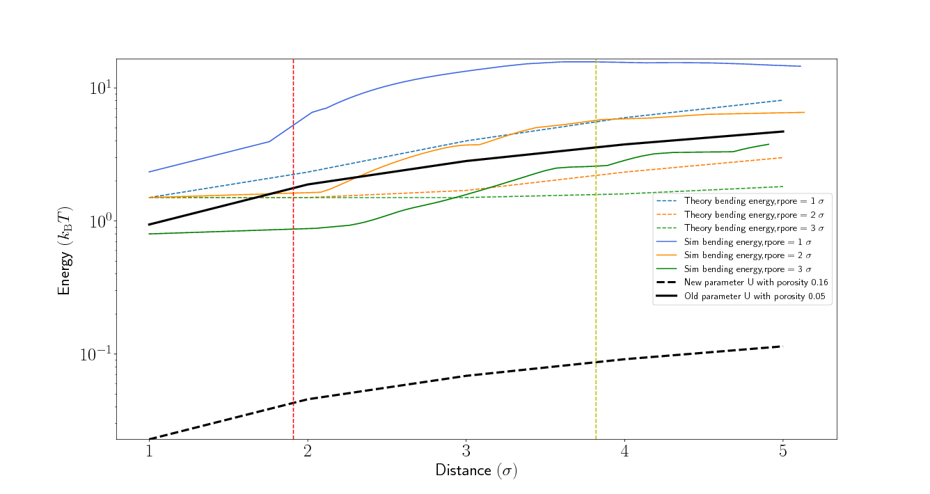
In the above figure we can see the results of the computations. The vertical dashed lines correspond to the bounds on our toy model for bending. The reasoning behind them is that since the hyperbola can’t bend anywhere other than the middle it can’t capture any conformation where the free ends of the chain bend significantly. This implies that the bending energy is valid until a few Kuhn segments have moved to the trans side of membrane (the two lines correspond to a different number of Kuhn segments). The simulation results for the bending energy confirm that our model gives us a good approximation for a chain folding.
As expected, the potential energy in a typical pore due to the applied voltage is not enough to bend the molecule through the pore with the new parameters. This was quite puzzling as successful events were registered at the sensing pore in experiments.

One hypothesis as to why this might be happening is that we used average pore sizes in our calculation. Given the large number of pores on the filter there must be some that are a few standard deviations away from the mean (assuming the pore sizes are normally distributed). Alternatively, there could also be anomalous pores on the filter. These anomalous pores would exhibit irregular or elliptical shapes which would allow their semi-major axis to be large enough to facilitate folding. Looking at the TEM images provided by Kyle Briggs (shown below) we noticed the presence of these anomalous pores some of which were as big as 100nm in diameter. Unexpectedly, the TEM images also illustrated the fact that our assumption of uncorrelated pore layouts was wrong and the pores do in fact form clusters on the filter. The major lessons to learn from these images is that the formation of anomalours pores is possible and that in their maximum dimension they can be a lot larger than expected.

Conclusions

Currently, our recommendation for more control over the device is to reduce the porosity of the filter as doing so allows for more uniform pore sizes. Furthermore, an overall increase in the filter pore size would increase the low capture rate exhibited by some devices.

We would like to do some further analysis on this in order to have more accurate parameters for our simulations so that we might have more insight on the dynamics of the device.  In particular we have been looking at the figure below (again provided by Kyle).

 

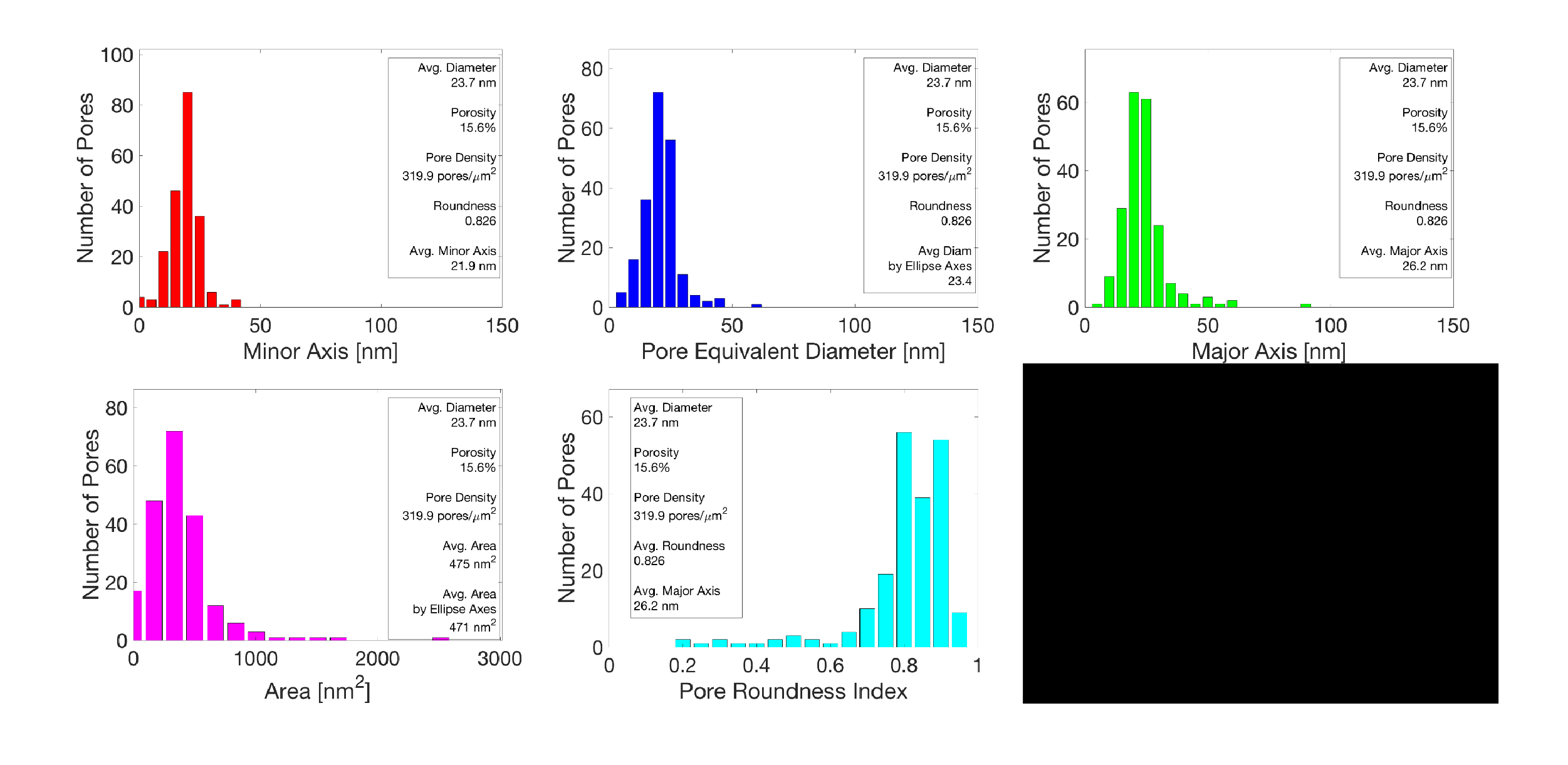
In order to better tune simulations to experiment we would like to be able to generate plots like the ones above. Specifically, we would need the TEM images and whatever tools are used to analyse them and obtain pore size distributions etc.