
Merging Man with Machine: A Computer Vision Aided Leukocyte Transmigration Assay
Introduction
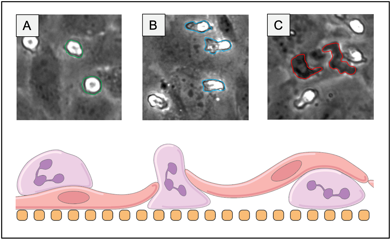
High throughput imaging techniques in conjunction with in vitro micro-physiological systems (MPS) allow for comprehensive exploration of physiologically relevant phenomena in a living 3D mimetic of a tissue microenvironment. Prior work in this lab has readily demonstrated that vascular tissue mimetics (the µSiM) facilitate real time phase-microscopy visualization of immune cell trafficking in response to inflammatory conditions. Our work with monitoring polymorphonuclear leukocytes (PMNs) on µSiM devices treated with a variety of inflammatory cytokines generates large volumes of imaging data. Processing such data by hand is tedious and time consuming, especially noting that manually counting/tracking PMNs is subject to a high degree of bias. Mitigating such tedium requires incorporating a robust computer vision aided approach, noting that conventional image processing algorithms are incapable of assessing multi-phase leukocytes (Figure 1). Therefore, companion machine learning and computer vision technologies must be concurrently developed to enable the processing and interpretation of microscopy studies capable of generating massive data sets.
This post serves to detail the progress made thus far with respect to our work with developing a computationally assisted, label free, short term leukocyte transmigration assay.
Methods
Device Fabrication
Initially, we attempted to adapt the modular µSiM flow unit created by collaborators at RIT. Unfortunately, we encountered several issues when attempting to adapt the flow unit towards static studies with NPN so hand-built devices were created instead (Figure 2).
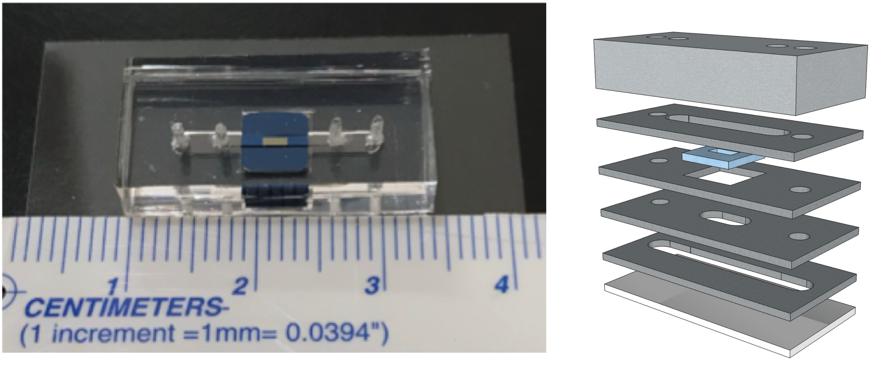
These devices require a more arduous fabrication process versus modular µSiMs provided by ALine. We’ve discussed this procedure multiple times (e.g., Alec and Kilean’s posts) and we’ll go over it once again for the sake of repetition. The layers and composition of this device are as follows (in order of assembly):
Layer 1 (base and imaging support): Glass Coverslip, 24 x 40 mm (Corning, Corning, NY)
Layer 2 (bottom channel): 130 µm Tape (Adhesive Transfer Tape 468MP, 3M Corporation, St. Paul, MI)
Layer 3 (membrane sealing layer): 300 µm Silicone Gasket (Custom Silicone Sheeting/Film, Trelleborg Sealing Solutions Americas, Fort Wayne, IN)
Layer 4 (membrane layer): 300 µm Silicone Gasket
Layer 5 (top channel): 130 µm Tape
Layer 6 (support block): Polydimethylsiloxane (SYLGARD™ 184 Silicone Elastomer, DOW Chemical, Midland, MI)
Briefly, layers are cut to size according to a diagram via craft cutter (Cameo 4, Silhouette America Inc., Lindon, UT) and assembled around an NPN membrane (SiMPore, West Henrietta, NY) in the aforementioned order (note, upon addition of layer 3 the device is autoclaved). The PDMS layer is manually cut with razor blades and 1 mm biopsy punch. Gasket layers, membranes, and PDMS are UV ozone treated (15 minute exposure w/ 2 hrs in a 70 degree furnace). Devices are sterilized in a cell culture hood via UV light before culture.
Cell Culture and PMN Isolation
Both of these processes are described in detail in Alec’s recent paper: click here to access it.
Check the materials/methods section for more information.
Machine Learning Algorithms
Two algorithms were utilized in this study, one to create a color coordinated pixel map (semantic segmentation) and another to interpret those results (object classification). WEKA (via random forest algorithm) provided semantic segmentation data while LENet-5 (via a convolutional neural network) provided interpretation of the semantic segmentation results. I have discussed the development of WEKA based algorithm in more detail in earlier posts here and here. To recap:
FIJI supports the WEKA segmentation plugin that allows for ground truth labeling of images, feature selection, model training, model generation, and subsequent classification through a headless interface via terminal (or command prompt). All of the image processing performed for this work was done with multiple computers. As WEKA does not support graphics processing unit (GPU) acceleration, central processing units (CPU) were exclusively used for computational processing. The main computer used (CPU/RAM/GPU/OS) is as follows:
Ryzen 9 3950x, 64gb DDR4 RAM, Nvidia/EVGA RTX 2070 Super, Windows 10
Beanshell, ImageJ Macro language, and Batch were utilized for scripting, implementation, and automation of the machine learning process via WEKA. Mathematica via Wolframscript was used for data analysis, video correction and plotting. Ground truth labeling was performed in FIJI, with labeled regions saved via “ROI Manager” (Figure 3). Four classes were established in order to differentiate neutrophils and HUVECs, and images were sourced from brightness corrected frames from all experimental conditions (Pos/Neg control, Luminal/Abluminal TNF-alpha, and fMLP). Neutrophils could be in “phase bright” (bright white), “probing” (gray), or “phase dark” (transmigrated, black) while HUVECs were given one class: “endothelial background”. Emphasis was placed on labeling boundaries between classes in ambiguous cases. The four classes were pixel balanced in order to prevent overfitting for one class and multiple features were utilized in order to enhance the model. These include: Gaussian blurs, Sobel filters, Hessian matrices, Difference of Gaussian, Membrane Projections, Mean, Minimum, Maximum, Variance, Entropy, and Neighbors. The mathematical descriptions of these convolutions are described in the ImageJ wiki.

After labeling, models were trained and saved as both “.arff” files (containing ground truth labels/traces) and a “.model” file that was used for video classification. A beanshell script was adapted from the ImageJ wiki in order to process frames of a video separately in order to mitigate memory issues.
The LENet-5 convolution neural network (CNN) was intended to solve the issue of counting PMNs when they cluster in a video. The LENet-5 CNN was initialized, trained, and deployed in Wolfram Mathematica. A training data set of n = 27,200 labeled examples split equivalently across two classes, single PMN, and multi PMN, was trained on semantic segmentation data from the WEKA model. Data was taken from classified videos of devices featuring ‘dual scale’ membrane materials and several permutations (e.g. rotations, mirroring) were applied to ground truth labels to increase the number of training examples. Subsequent counting of PMN clusters/detections was performed via post-hoc scripting. The following figure depicts an overview of the image analysis pipeline (Figure 4):

Tracking was performed by utilizing a nearest neighbor linking (NNL) approach (Figure 5). The script modified the validated PMN counting script by incorporating additional data and logic necessary for tracking. Centroid data for all detected objects in frame was tabulated to a tuple, and custom scripting used to assign tracks across a video.
Multiple corrections were made to eliminate common issues with tracking such as trajectory repetition and jumping. Other issues such as trajectory trading and fragmentation were minimized. Upon collecting as many tracks as possible, tracking data was fit to an equation relating mean squared displacement to “speed” and “persistence” values attributed to mathematicians Dunn and Othmer (henceforth referred to as the Dunn Equation, Equation 1). Speed is simply a measurement of displacement over time while persistence is a measure of directional bias over time in an indirect measurement of cell polarity. For the purposes of model validation, speed/persistence values from curve fits were obtained from fragmented track lengths. The time gap “tau” was set for minimum value required for convergence such that tau was close to persistence time. Doing so minimizes the need to discuss the linear form of the Dunn equation, which is necessary when tau >> P. These curve fits from model data were then compared to curve fits performed on manual tracks (n = 15 neutrophils per video).
EQ. 1: D = 2S2(P t -P2(1 – P e-t/P)
Statistics Overview
In order to assess model accuracy, we sought to achieve statistical parity between the model and manual tracking for two key metrics: number of PMNs counted in a frame and transmigration ratio results based on bulk pixel data (note, PMN count also has an attached <10% error metric associated with it). For PMN count, a Chi-squared goodness of fit test was performed while an unpaired t-test was utilized for transmigration data. For transmigration data, we opted to analyze “equilibrium regimes” in which PMNs appear to have achieved a steady-state response to a chemical stimuli (Figure 6). A Chi-squared analysis is not possible on transmigration data due to the presence of zeroes in the denominator for expected values (i.e. no transmigration).

Manual counting of PMNs was performed on the first frame of a video, followed by every 30th frame (i.e., 1, 30, 60, 90, … , 450) where both apical and basal PMN populations were tabulated. Statistical comparisons for tracking data, PMN counting, and transmigration ratios was subsequently performed.
Results/Discussion
Original Analysis with Older Data and Post-Hoc Scripting
Initially, we sought to apply post hoc scripting and particle counting techniques (logistic regression) to the high contrast pixel maps generated from the semantic segmentation algorithm. Generally speaking, the algorithm under-counted PMNs when operating under this method (Figure 6).
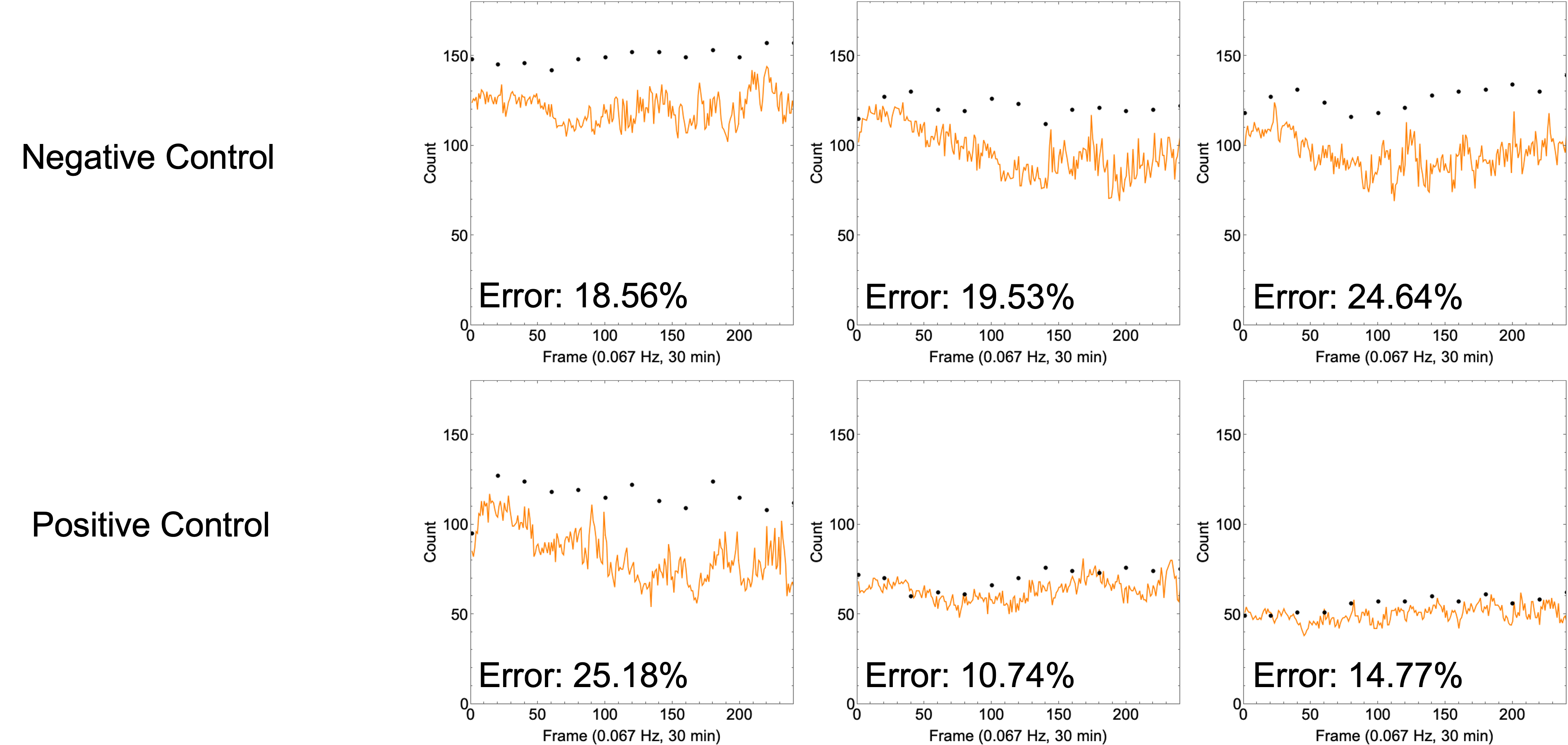
None of the measurements achieved our success metric of <10% error, however we did note that lower PMN counts coincided with lower error rates.
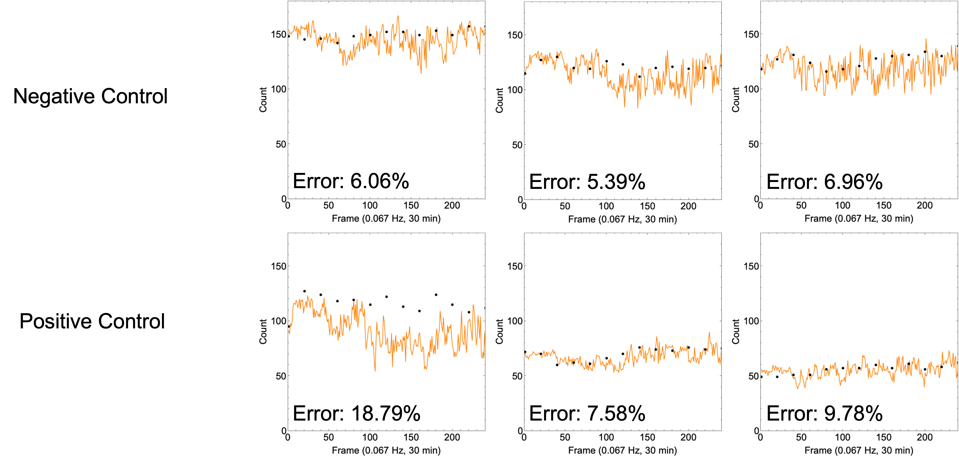
We then applied the LENet-5 CNN for assisting with counting PMNs, and our accuracy increased dramatically, although the variability in detection was still high (Figure 7).
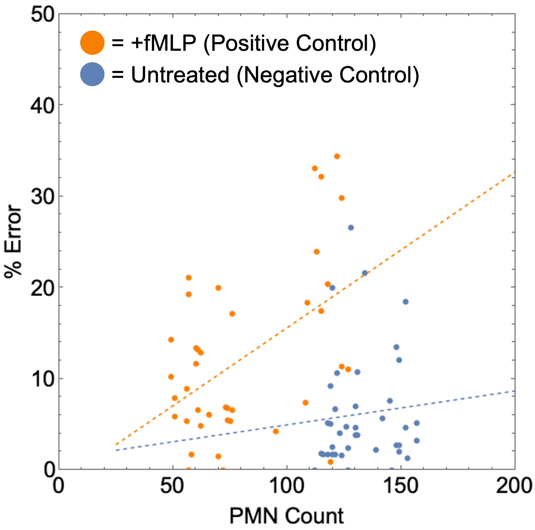
When percent errors are plotted in a scatterplot and fit to linear regressions, we find that both positive and negative control experiments can achieve high accuracy (<10% error) by keeping PMN counts in frame low (~40 or infusing 20 µL of PMN rich media at a density of 3 million PMNs/mL) for both conditions (Figure 8).
New Dataset (n=3) +/- Control
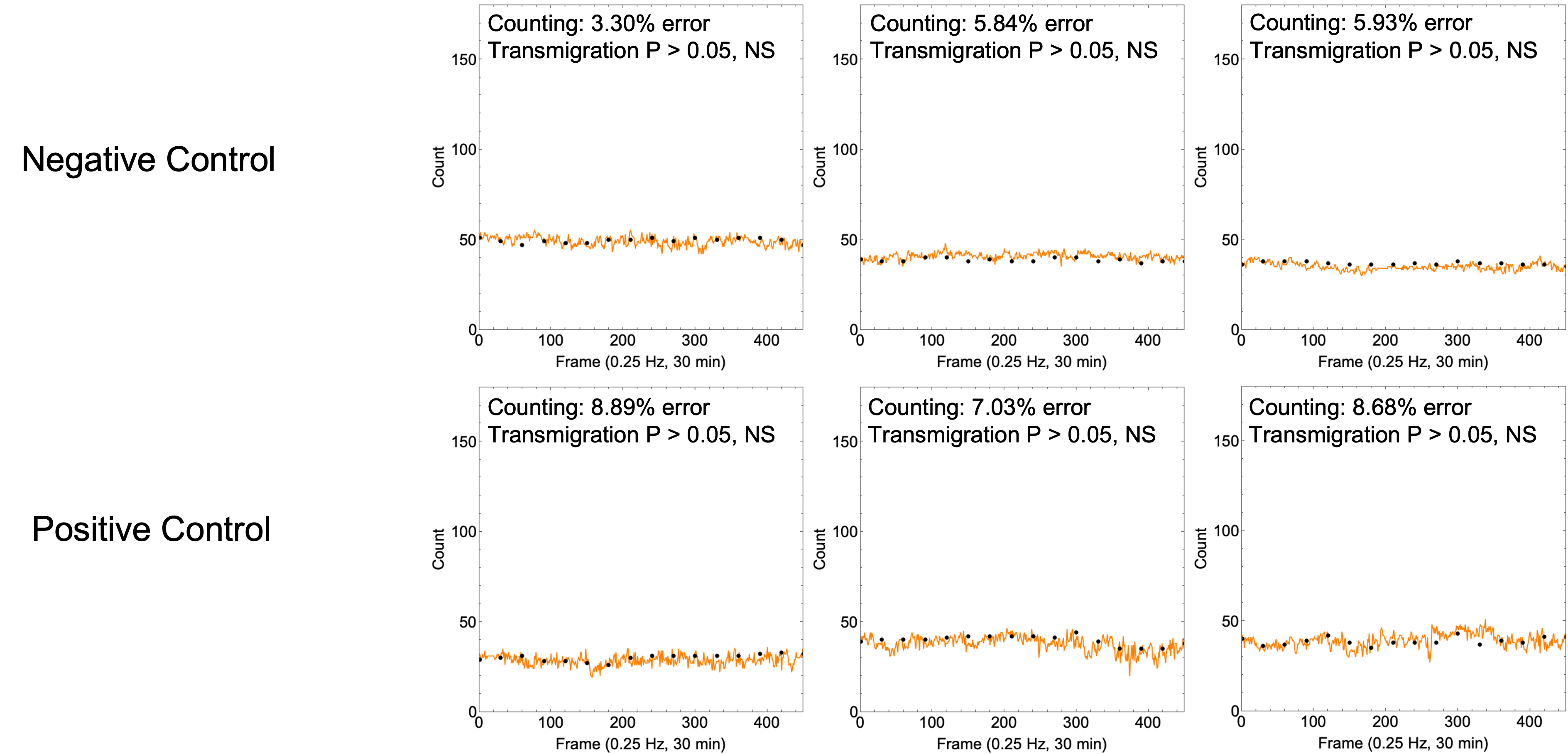
Redoing the experiments with controlled seeding densities resulted in high accuracy counts with low variability (Figure 9).
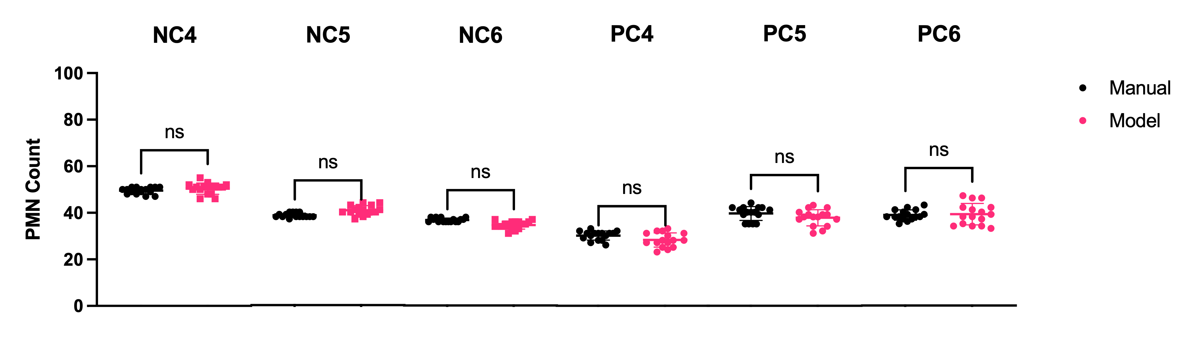
When statistically analyzing model counting versus manual counting with a chi-squared goodness of fit test, we find robust statistical agreement across all conditions surveyed (Figure 10).
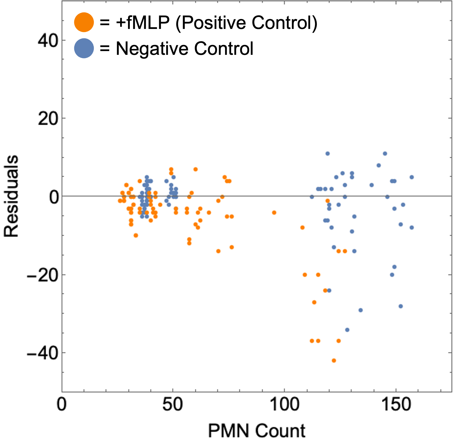
When analyzing residuals across all data gathered thus far, we find that the lower PMN count experiments have more distributed residuals while higher PMN counts tend to result in under counting (Figure 11).
Transmigration results also displayed statistical agreement between manual counting and model counting (Figure 12).

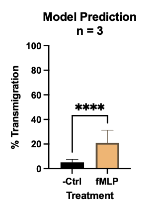
Comparing overall transmigration ratios between positive and negative controls depicts clear activation as a result of fMLP stimulation (Figure 13), as expected.
NNL tracking data of the positive and negative control studies depicts a robust difference in migratory activity based on tracks alone (Figure 15).
Despite the robust tracking capability, a key limitation of our current algorithm is that we are unable to assign a PMN identity to a particular trajectory. This is due to a limited axial resolution in 2D phase contrast imaging. When a phase dark PMN and a phase bright PMN travel over one another, there is a possibility of losing a track. This does not always happen, however, and appears to be a sporadic event.
Trajectory Collisions: No Trading
Trajectory Collisions: Trading
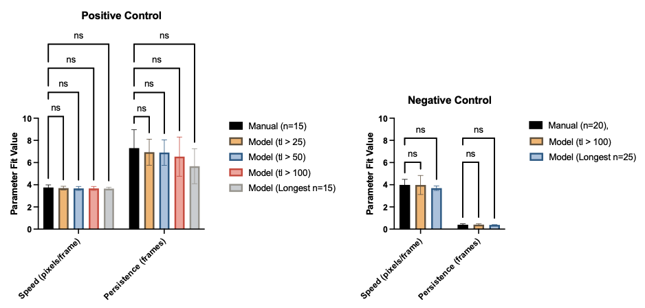
Despite this, the presence of sufficiently many tracks results in statistically similar speeds and persistence data between models and manual tracking (Figure 16).
When comparing positive controls to negative controls (tl > 100), we find that speeds are similar but negative control PMNs are less persistant (Figure 17).

We can also calculate the chemotactic index (CI), which is displacement from origin divided by path length. A lower CI implies less chemotaxis and is analogous to persistence. The model is capable of calculating statistically similar CI’s when compared to manual tracking (Figure 18).

Conclusion and Future work
With this validated model, we can now perform state analysis/tracking of PMNs in a video for a given stimulation. We have already started evaluating the effects of apically oriented cytokine stimulation with a “cytomix” blend of equimolar TNF-a, IL-1b, and IFN-g. These results will be the topic of a future post.