Generating COMSOL Simulations of Actual Pore Geometries

As Greg posted last time, he and I have been working on a manuscript for all of the tomography stuff that we have done that we are going to hopefully submit this week. In that paper, we covered all the tomography techniques that Greg uses to reconstruct models of the pores and then used these models in the computational fluid dynamics (CFD) simulation software COMSOL. As Greg has already posted about his reconstruction techniques, it is now appropriate that I post on the reconstruction and simulation of these actual geometries in COMSOL.

The tomographic reconstruction process generates STL files, which are a standard 3D printing file. It represents an object as a mesh and is a relatively simple structure. It does not contain solid information about the object and therefore some transformations have to be performed in COMSOL. As a base package, COMSOL has the capability to import these STL files as a mesh and which can then be converted to solid objects (Figure 1).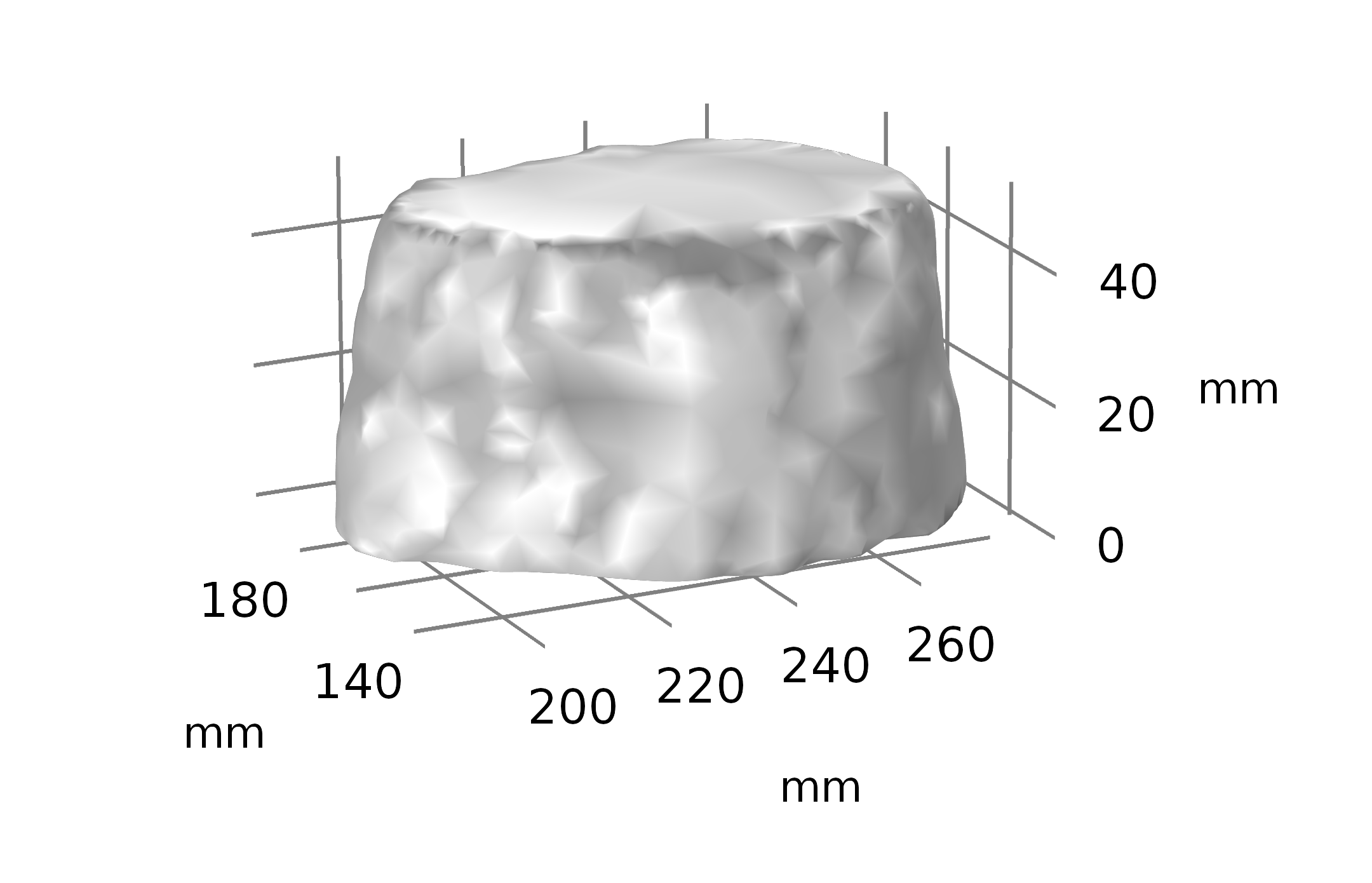

Figure 1: Imported STL pore in COMSOL. Note the lack of defined faces and boundaries.

However, this method is not fully comprehensive as it is reliant on the initial mesh file being accurate. If there are any errors, no matter how minor, the modeling process fails because of the inability of COMSOL to correct and account for these errors. Self-intersecting faces and non-manifold edges present the largest problems as they present geometry decomposition errors when trying to combine the pore(s) with simple COMSOL geometry objects. As noted in Figure 1, these simple manipulations are necessary to help to define faces for flow into and out of the pore. Without these, the pore is one object and can only be set as one condition. In order to fix this then, I had to transform the initial pore geometry that we used from the base STL file. The program that Greg uses generates these pores as high complexity meshes sometimes with over 1 million elements per pore (Figure 2).

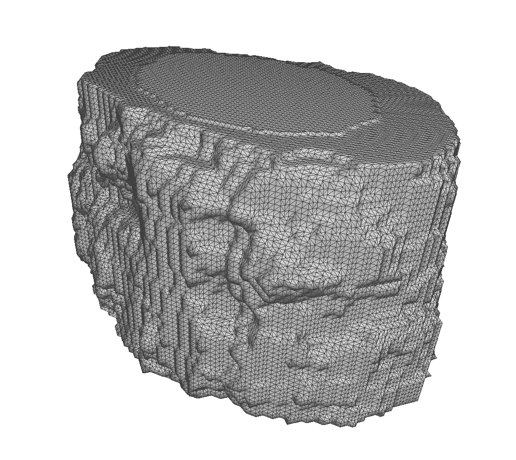
Figure 2: Complex Pore rendered in meshlab. This pore contains 54,500 faces.

While this is very good for rendering and understanding the full structure of the pore, it is inconvenient when trying to import the file into COMSOL. The number of elements causes the formation of overlapping entities and errors. Therefore, I had to first reduce the number of elements in the geometry to simplify it for import. I took a pore that had 54,500 faces initially and then used the program meshlab to reduce the number of faces to 1000 using a Quadric Edge Collapse Decimation filter (Figure 3). This drastically simplified the model but still retained the majority of the features of the pore that would be interesting during simulation.

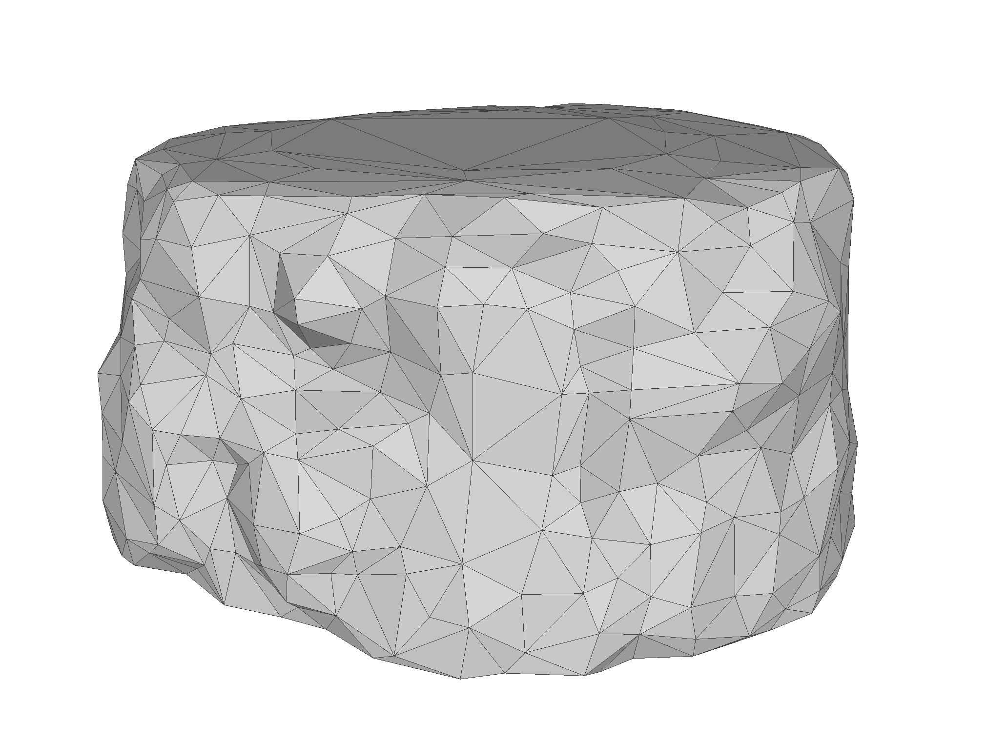
Figure 3:  Pore rendered in meshlab. This pore contains 54,500 faces.

With the simplified model, I was then able to reimport the mesh into COMSOL and I removed all the errors that I was previously getting. I was then able to perform several operations on the pore which allowed me to generate faces to set as inlets or outlets. Specifically I created two block objects and overlapped them with the top and bottom 3 mm (nm) of the pore (Figure 4). I then used the partition objects feature of COMSOL and partitioned the pore with these two blocks, creating two planes within the geometry (Figure 5). I was then able to use block objects in the place of the original partition blocks and perform a difference operation that removed the top and bottom 3 mm (nm) of the pore (Figure 6).

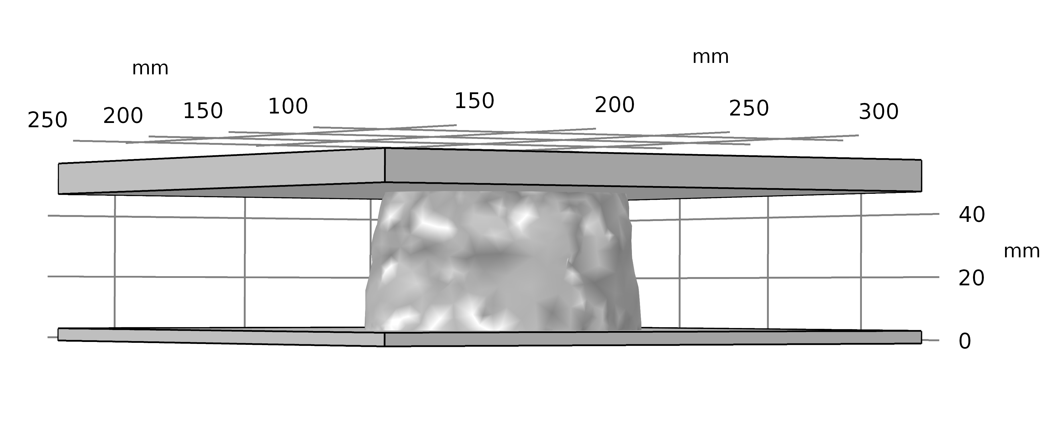
Figure 4: Blocks used for partitioning the pore object.

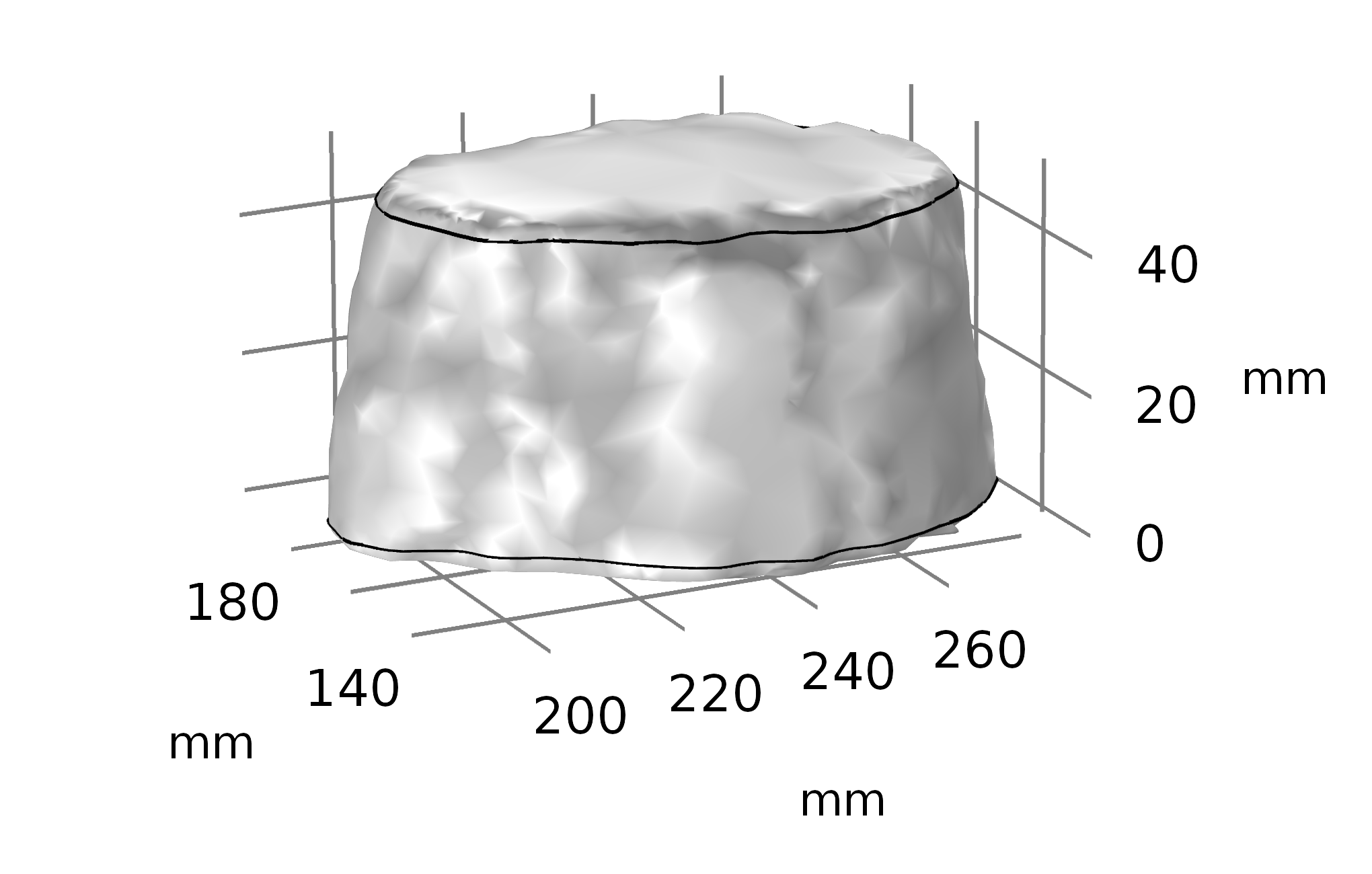
Figure 5: Partitioned pore.

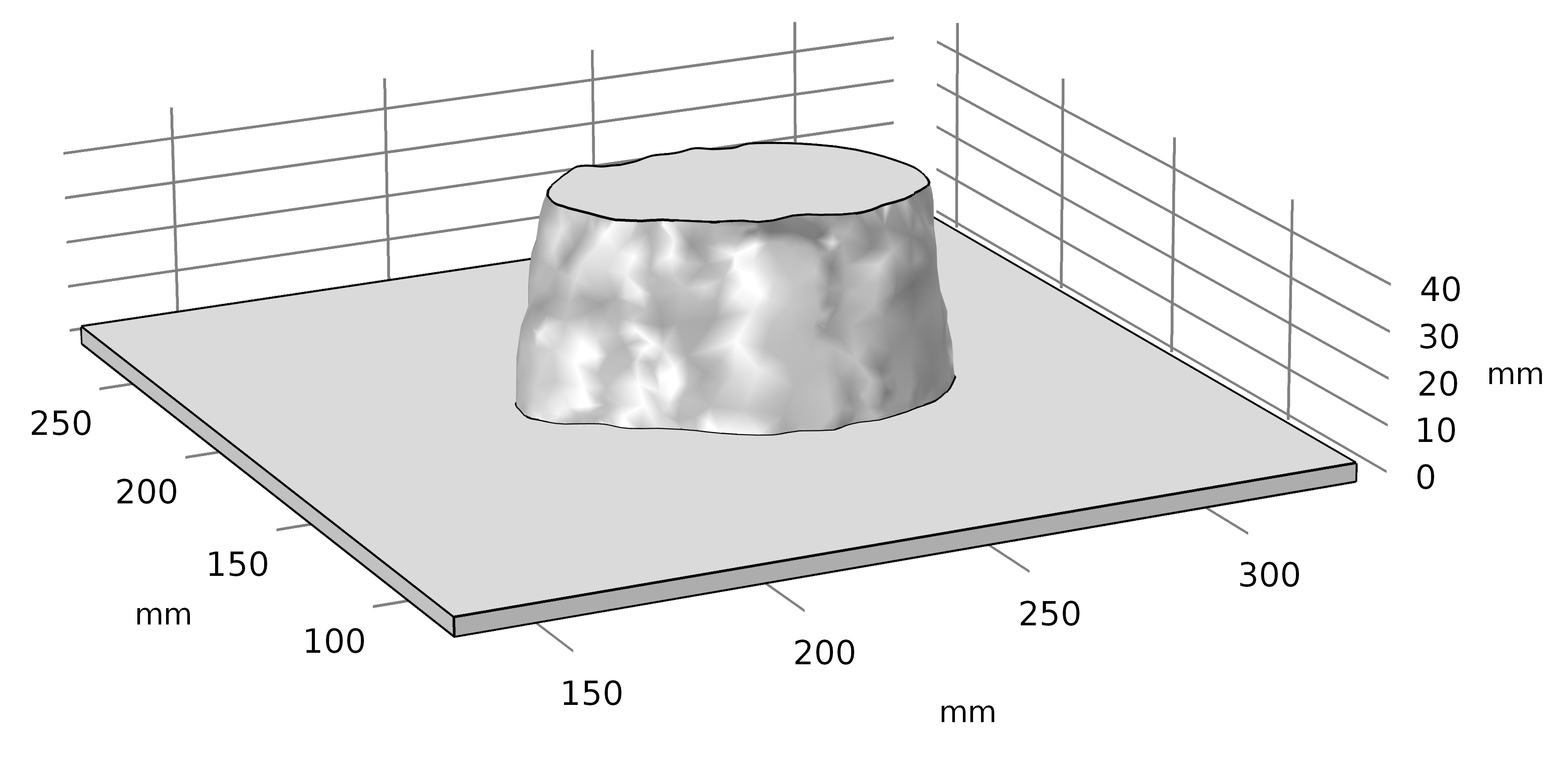
Figure 6: Pore with top portion removed to set a face for modeling.

With these operations out of the way, I applied physics to the geometry and ran a steady state, laminar flow study. I used the conditions that I would normally use for exosome capture (10 μL/min) and calculated the velocity through an individual pore (5.7e-5 m/s). One of the surfaces was set as the inlet with a velocity condition and the other was set as an outlet with a pressure condition (zero gauge pressure). The simulation was run both wide to narrow and narrow to wide (what we would define as top to bottom and bottom to top). As we can see in Figure 7 and Figure 8, the structure of the pore plays an important role in the simulation. The nanofeatures of the pore contribute to the boundary layer quite significantly and can potentially explain capture events that we observe where there should not be any capture. However, these low velocity pockets are regions in which particles or proteins can stick within the pore. A cylindrical pore would fail to capture these features (Figure 9), thus showing the limitations of working with simplified geometries.

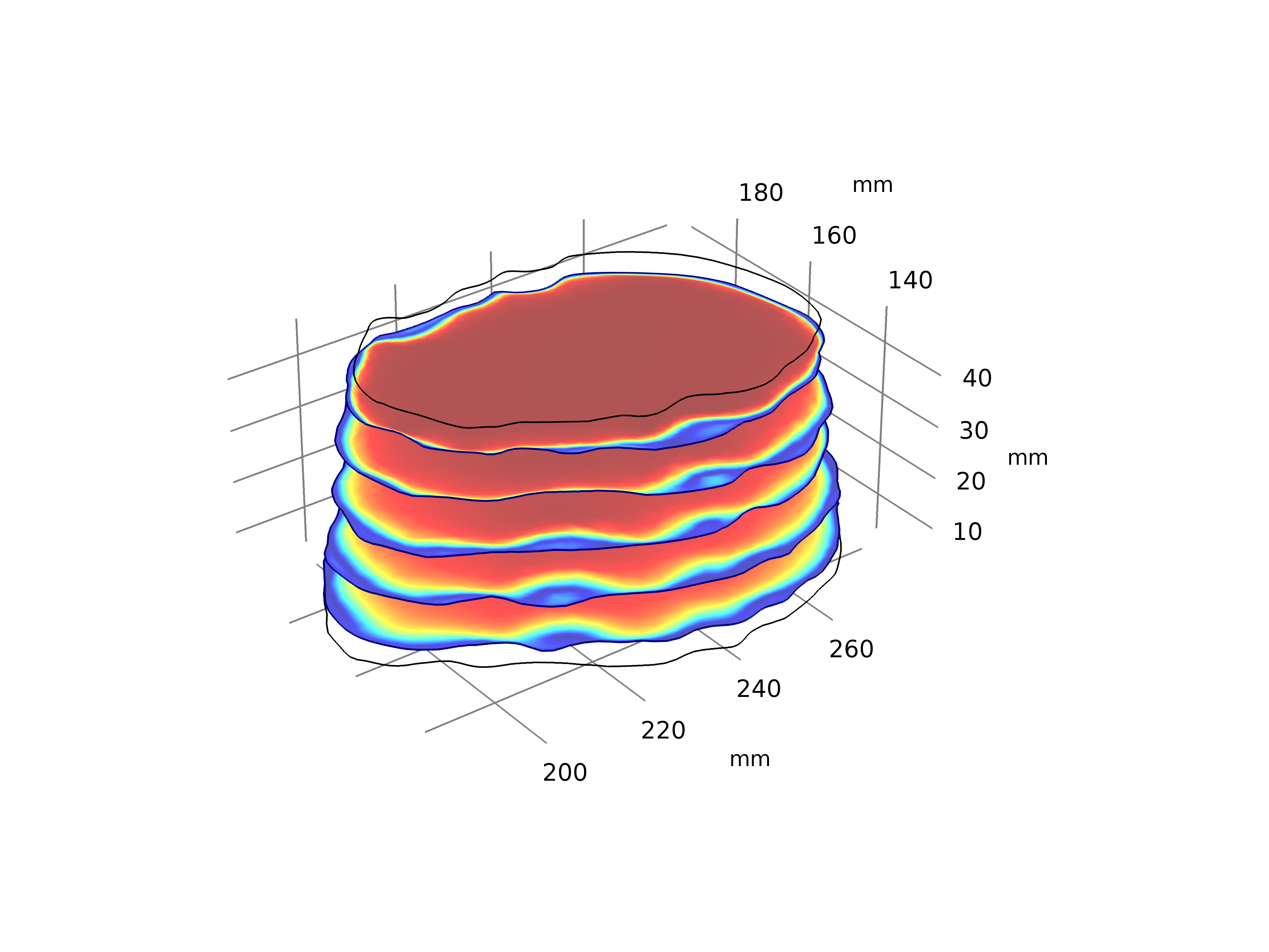
Figure 7: Fluid velocity simulation of an actual pore run from bottom to top.

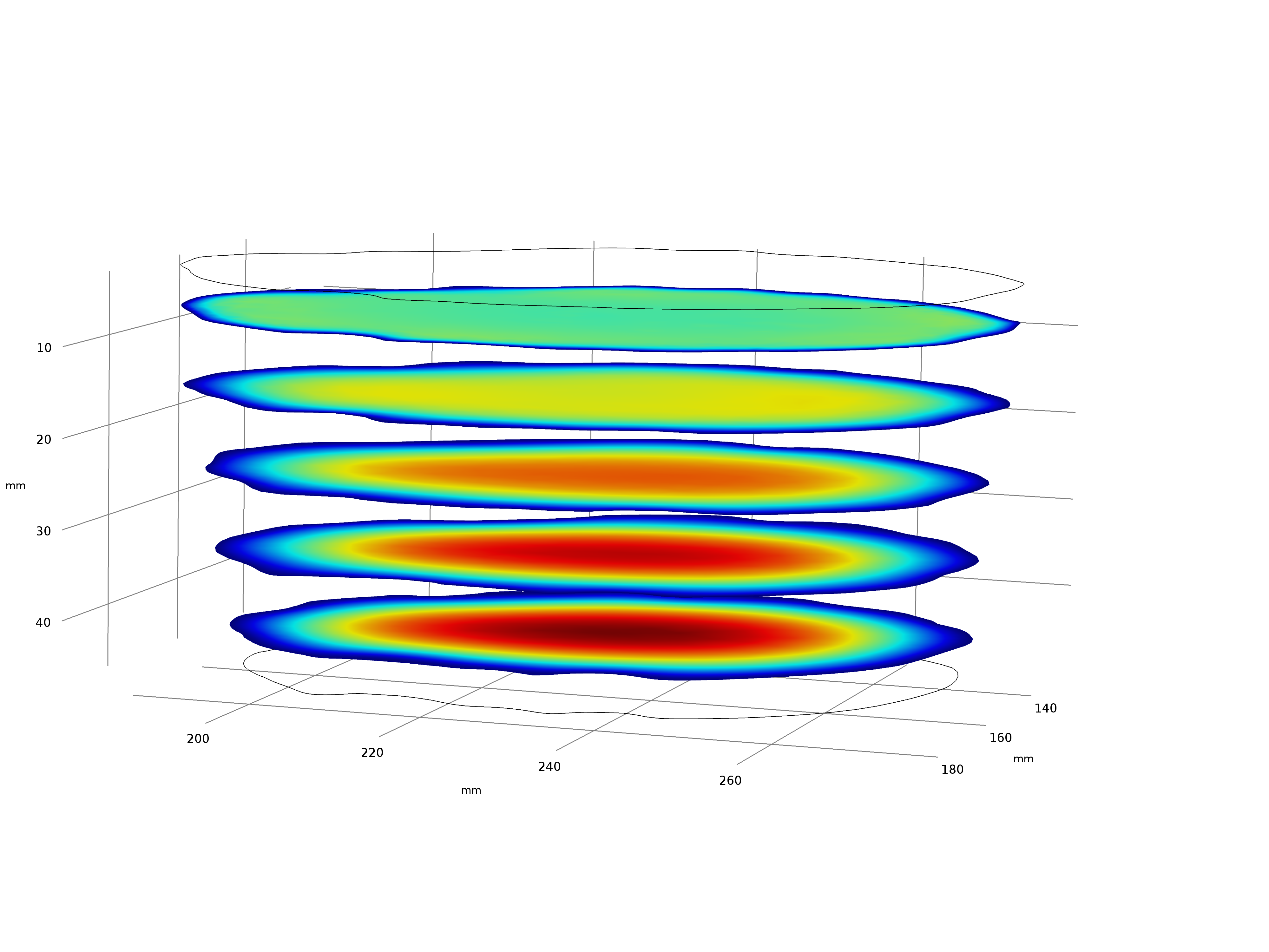
Figure 8: Fluid velocity simulation of an actual pore run from top to bottom

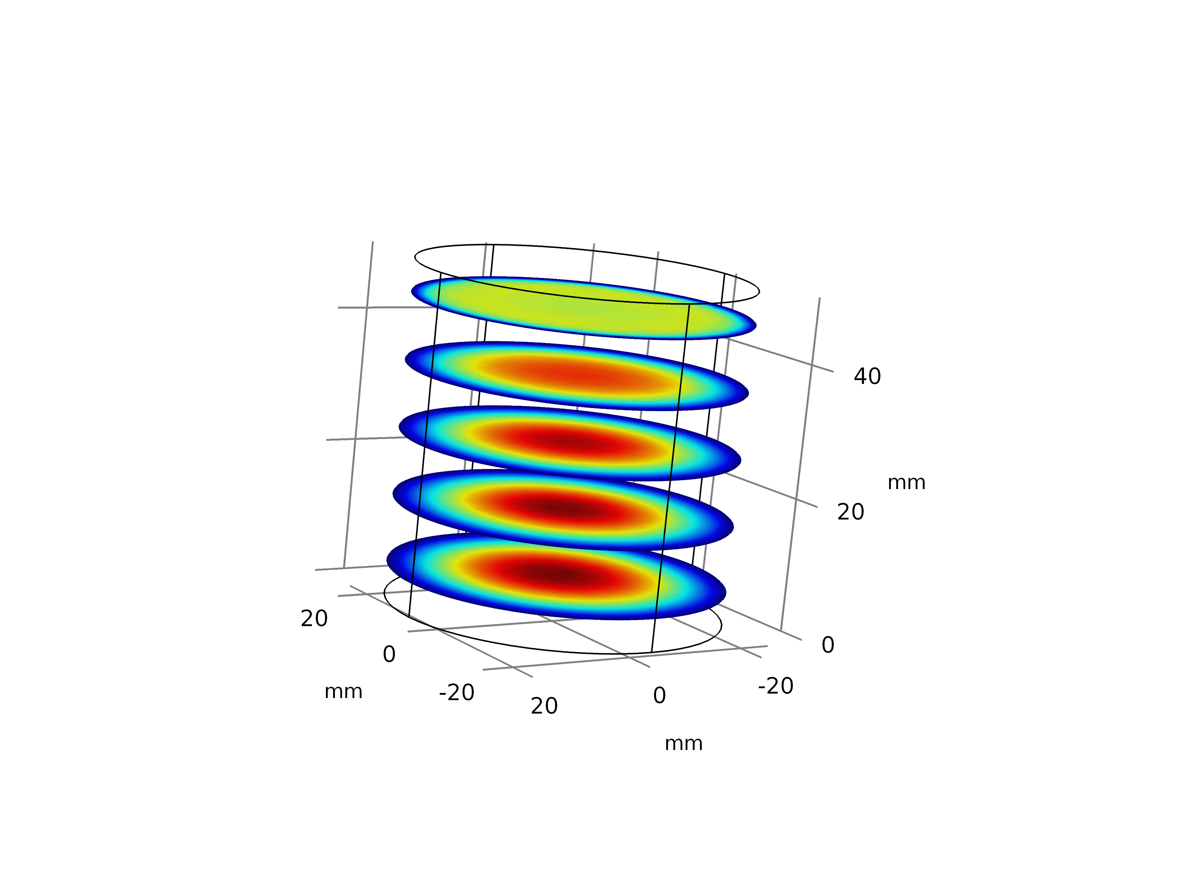
Figure 9: Cylindrical pore with equivalent flow conditions as the actual pore.

Now this whole analysis was interesting and all, but the ultimate question was whether or not we can model more complex pore geometries. So, I tried this. Greg found a bifurcated pore on a membrane from wafer 1272 and I attempted to perform the same operations that I had to import the simpler pore. However, there were significantly more errors with this pore and I was unable to import the STL file and perform any operations on it. I then turned to somebody with CAD experience to possibly help me out with repairing the file and converting it to a solid object. Now, with our new version of COMSOL, we had purchased the CAD Import Module, so I tried saving the file to a DWG or SLDPRT format, but unfortunately, it would appear that COMSOL is super stupid and frustrating and those extensions only work with the Windows version of COMSOL for importing. So at this point, I threw out $5000, brand new iMac Pro off the third floor and gave up on this whole idea.

Well…..I didn’t quite do that, but I was very frustrated at this point as this has been a problem that Dean has been having as well and it was very annoying. So I looked in the documentation at the file types that the CAD Import Module COULD import on Mac and found that we could work with an IGS file type. So I asked and was able to get the pore as a CAD file in the IGS file format. I imported this into COMSOL and was able to successfully perform this operation. There were some minor errors that I had to clean up once in COMSOL, but I was otherwise successful in importing this object (Figure 10).

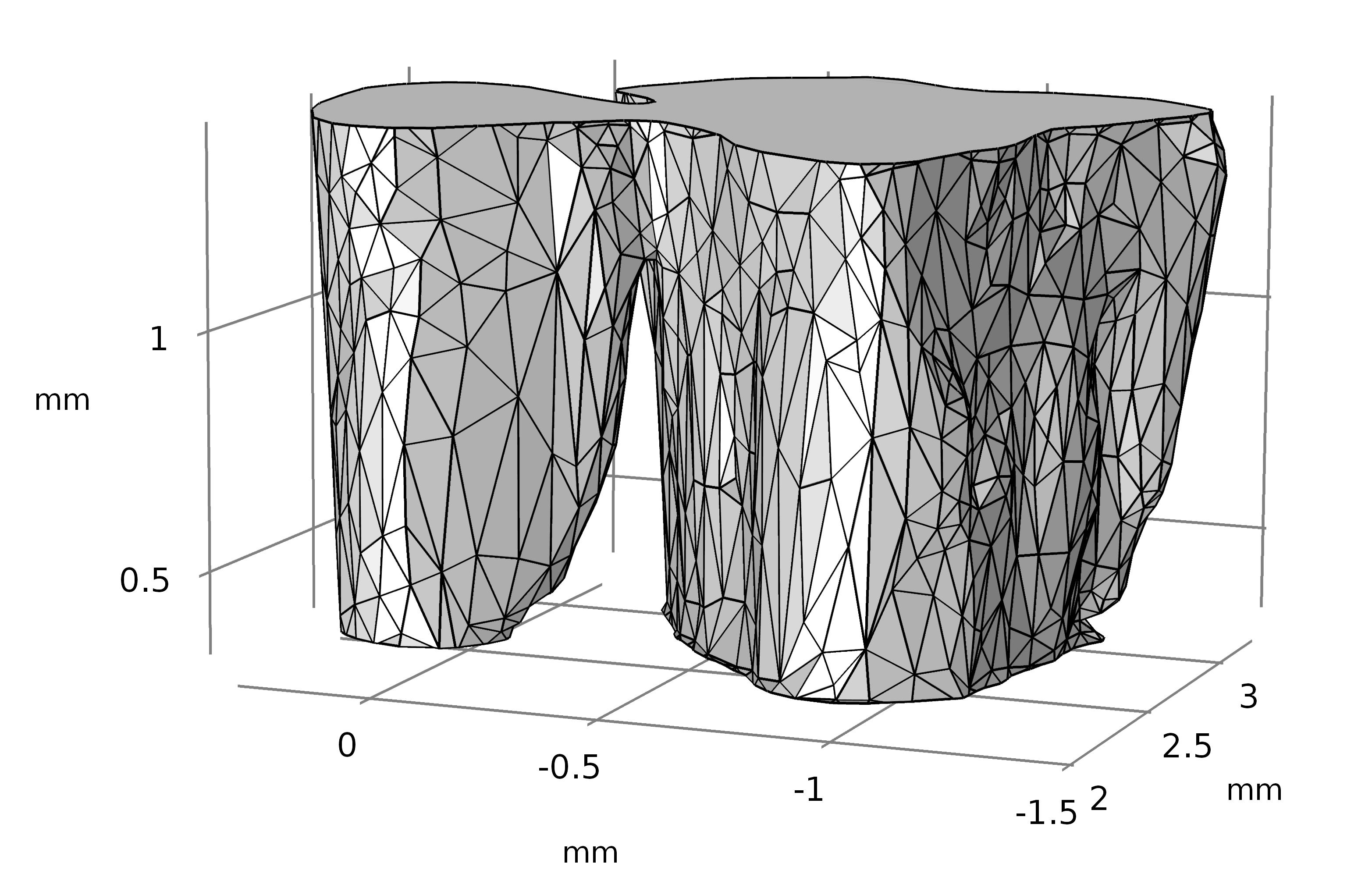
Figure 10: Bifurcated pore imported into COMSOL

I performed the same simulation on this pore, with the exception of running this reversed: I only ran it from top to bottom. As we can see in Figure 11, the complexity of the pore showed things that we wouldn’t see with a standard cylindrical representation. This is best seen in Figure 12, where I use the interactive slice feature to look at the velocity in the yz-plane.

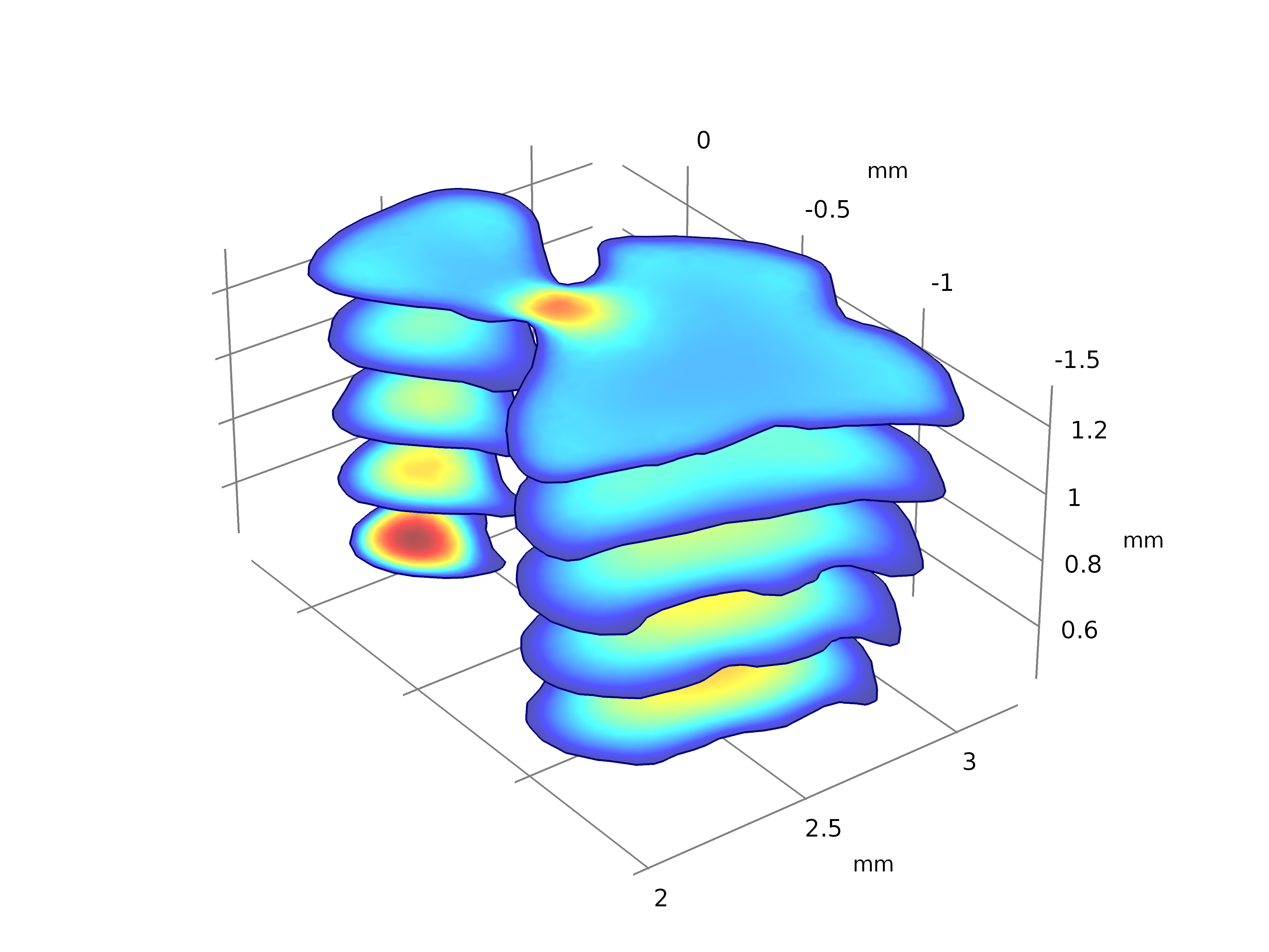
Figure 11: Bifurcated Pore velocity simulation.

Figure 12: Interactive velocity slice look at the velocity through a bifurcated nanopore.

This technique is now at the point where we can implement modeling of individual pores with geometries that actually represent the structures we have in our membranes rather than simplified representations. This enables fluid flow, particle capture and electrical field simulations with more realistic results.