Sieving Model 2.0 Curves for Varying Gold Concentrations, Membrane Thicknesses, Salt Concentrations, and Applied Pressures

These curves were all generated using the following package of matlab functions and scripts: (Sieving copy – run Find_Sieving_Coefficient_boltzmann.m – it’s set up to generate concentration profiles right now).

The program begins with a ‘standard separation’ that uses the following characteristics:

Pore diameter: 58 nm

Particle diameter: increases from 20 nm to 56 nm in 2 nm increments

Pore Zetapotential: -20 mV

Particle Zetapotential: -15 mV

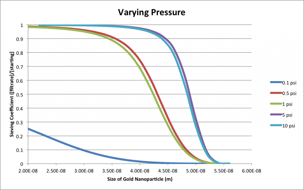
Transmembrane pressure: 3 PSI

Salt concentration: 0.001 M (KCl)

Membrane thickness: 50 nm

Approximate number of pores in a Sepcon chip: 400,000,000

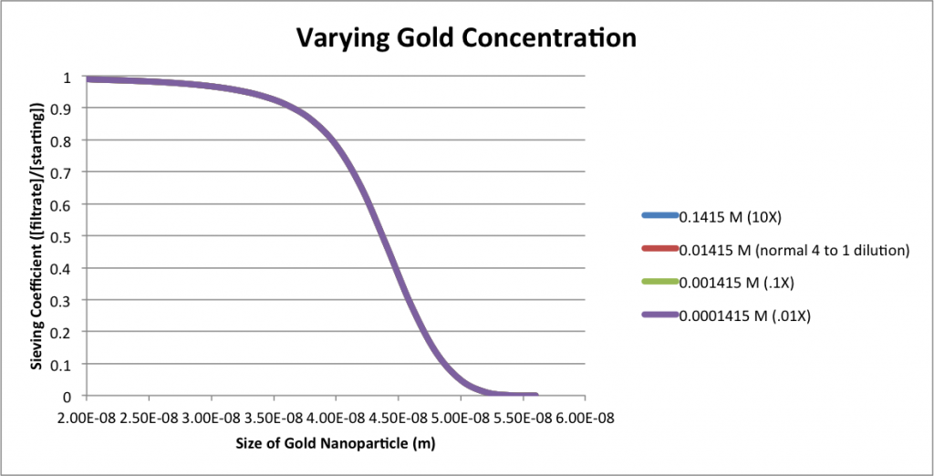
Starting gold concentration: .25* 5.66E-2 M (our standard 4 to 1 gold dilution for one of the stock golds – I don’t remember which)

The simulation runs until 200 uL of fluid has passed (it’s a little more complicated than that because it’s a 1-D approximation of the volume)

For each of these graphs, I changed one variable to one of 5 different values to generate the plots. Keep in mind that each data point takes ~ 95 seconds to calculate on my machine, each curve takes 95 * 13 = 1235 seconds to calculate, and each plot takes 1235 * 5 = 6175 seconds = 102 minutes = an hour and forty minutes. I’ve chosen to break the calculation up into 300 pieces, because some numbers I ran at the beginning suggested good convergence at that ‘resolution’, but to get better data I may need to increase that to 1000 or more, at which point I may be beyond the capabilities of my poor macbook.

Next steps: include real pore distributions, and model the increase in hydraulic resistance coming from concentration polarization.

EDIT: The thickness curves I generated contain an error. Flow through individual pores is calculated using the famous Dagan equation (sometimes we also call it the Tong equation) which is used for calculating pressure-driven volumetric flux through a cylinder with an aspect ratio approaching 1 (where the diameter equals the height of the pore). But for the 10 nm thickness case, a 56 nm pore that is 10 nm thick can not have it’s hydraulic permeability determined via Dagan – the equation only works for cylinders longer than they are wide. So ignore the 10 nm curve. I ran some more simulations at much higher resolution – 600 iterations instead of 300 – albeit with a fewer number of gold particle sizes:

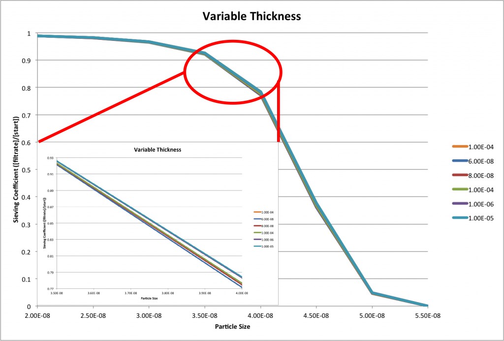
As you can see, the model barely predicts tighter cutoffs with thicker membranes, but the effect is far less pronounced than it was before. I think Jim is on to something in his comment below – we need a better model of what the high concentration at the membrane surface is doing to the separation. There are two components to this – the first is that we need some idea of how willing the gold is to concentrate – is there a maximum concentration it can achieve, after which adding more gold simply increases the size of the maximum concentration zone? (My hunch is yes). If that is the case, adding that to the model will change the separation characteristics. Further, I need to recalculate the hydraulic resistance of the gold nanoparticle layer at each step of the separation.