A New Update in the Particle Capture Saga
In this edition of the particle capture saga (this will eventually be an epic like Gilgamesh or Beowulf, we will start telling this tale by the fire and eventually thousands of years from now scholars will look back on this work and deem it a huge impact in the history of human evolution), I have finally succeeded in coupling modeling flow and particle tracking for a single channel parametric sweep. With virtually no help from COMSOL support, I generated a model (Figure 1), ran Free and Porous Flow, did a parametric sweep over top channel height, top channel flow rate (1-10 μL/min), and bottom channel flow rate (0-10 μL/min) and then ran a Time-Dependent Particle Tracing simulation where the particles were properly associated with the correct geometries and flow rates. All-in-all, this simulation had 662 different combinations and took a grand total of 27 hours to run on the iMac Pro (a smaller version of my final simulation). While I have a massive data set that allows us to visualize things happening in the system, I will postpone showing that data until the next time we have NRG at UR (we will hold it in a location that allows us to visualize the data in cool ways). Instead, today I will talk about some capture statistics.

Figure 1: COMSOL representation of simulated device. The model is completely to scale except for the thickness of the membrane.
One of the more powerful features of COMSOL is the ability to count the number of particles residing in a boundary, which I used to count the number of particles that I captured on the membrane. I then took this data set and extracted it to Excel where I generated several plots to characterize the system. The first thing that I did was take the particle capture counts at a 1 μL/min bottom:1-10 μL/min top condition for all channel heights and plotted the percentage capture for different top channel flow rates and heights. I plotted the resulting figure as both a marked line scatter (to see trends) and a bar plot (to get a better appreciation of the statistics), as shown in Figure 2 and Figure 3.

Figure 2: Marked line scatter plot of particle capture for a 1 μL/min bottom flow rate with varying top channel flow rates and heights. As the channel flow rates become closer, the particle capture increases for all channel heights.

Figure 3: The bar graph of this data allows for easier interpretation of how channel height plays an effect on particle capture for lower flow rates. Indeed, what this shows is that for higher flow rates, the effect of channel height is reduced quite significantly.
I thought this data was neat, but then I was curious about the conditions that I currently use; specifically I was curious about how well the 10:2 condition worked for capture. In theory, if drag was the only thing contributing to capture, we would only expect 20% of the particles to be captured. However, I have set a condition for myself of 75% capture. So I plotted that data.
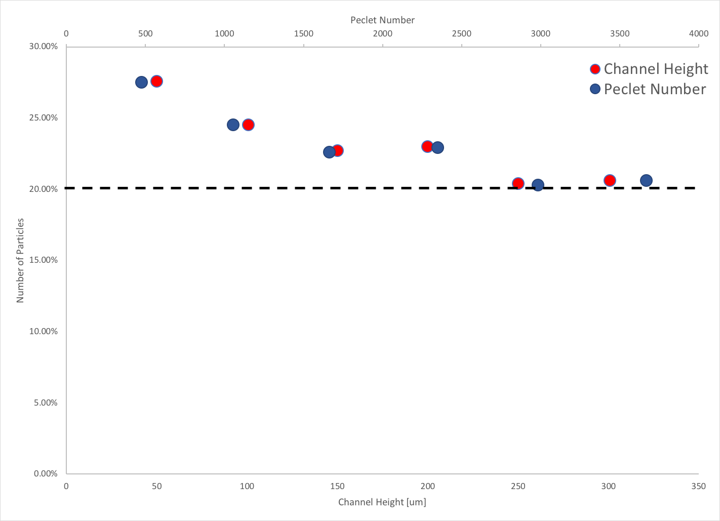
Figure 4: 10 μL/min:2 μL/min flow rate capture comparison for different channel heights and Peclet numbers. Note that there is always better than 20% capture, indicating that perhaps diffusion plays a part in the capture of particles under all conditions.
I then decided to explore how the Peclet number affected particle capture for a given bottom channel flow rate (this time I chose the 5 μL/min flow rate).

Figure 5: Particle capture as a function of Peclet number for a bottom channel flow rate of 5 μL/min.
In all this data, I have to be extremely careful: several of the combinations result in conditions where the bottom channel flow rate is higher than the top channel flow rate, which gives us a non-physical condition. Therefore, all these data points have to be thrown out.
While this is a robust data set, I have yet to go through everything and will be making more progress in the coming days. Eventually, I’d like to include plots with the flow rate ratios, to explore those effects, as well as understand capture at all the different conditions. Keep an eye out for those!